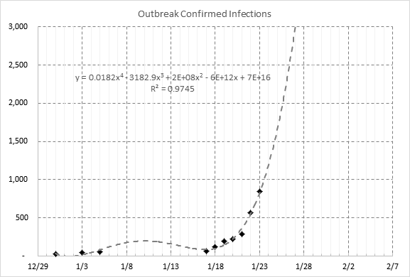
Forecasts are made based on live daily confirmation case data from the Chinese government since 1/31/2019. The case developing trend and case forecast for the next few days are shown in the graph below. The forecast line indicates the center of future data points, with a small variation.
Forecast for confirmed cases for the next few days are:
All measurements contain some uncertainty and error, and statistical methods help us quantify and characterize this uncertainty. This helps explain why scientists often speak in qualified statements. For example, no seismologist who studies earthquakes would be willing to tell you exactly when an earthquake is going to occur; instead, the US Geological Survey issues statements like this: “There is … a 62% probability of at least one magnitude 6.7 or greater earthquake in the 3-decade interval 2003-2032 within the San Francisco Bay Region” (USGS, 2007). This may sound ambiguous, but it is in fact a very precise, mathematically-derived description of how confident seismologists are that a major earthquake will occur, and open reporting of error and uncertainty is a hallmark of quality scientific research.
Today, science and statistical analyses have become so intertwined that many scientific disciplines have developed their own subsets of statistical techniques and terminology. For example, the field of biostatistics (sometimes referred to as biometry) involves the application of specific statistical techniques to disciplines in biology such as population genetics, epidemiology, and public health. The field of geostatistics has evolved to develop specialized spatial analysis techniques that help geologists map the location of petroleum and mineral deposits; these spatial analysis techniques have also helped Starbuck’s® determine the ideal distribution of coffee shops based on maximizing the number of customers visiting each store. Used correctly, statistical analysis goes well beyond finding the next oil field or cup of coffee to illuminating scientific data in a way that helps validate scientific knowledge.
Summary
Scientific research rarely leads to absolute certainty. There is some degree of uncertainty in all conclusions, and statistics allow us to discuss that uncertainty. Statistical methods are used in all areas of science. Statistics in research explores the difference between (a) proving that something is true and (b) measuring the probability of getting a certain result. It explains how common words like “significant,” “control,” and “random” have a different meaning in the field of statistics than in everyday life.
Key Concepts
Statistics are used to describe the variability inherent in data in a quantitative fashion, and to quantify relationships between variables.
Statistical analysis is used in designing scientific studies to increase consistency, measure uncertainty, and produce robust datasets.
There are a number of misconceptions that surround statistics, including confusion between statistical terms and the common language use of similar terms, and the role that statistics employ in data analysis.
The main goal of text analytics is to answer these five main questions:
Which terms and phrases are most common?
In what context are terms and phrases used?
Which terms tend to appear together? How an I group similar documents together and explore them?
What are the recurring themes (topics) within the corpus?
How can I reduce the dimension of the text data, so I can use the information in a predictive model?
Friendly user interface makes such analysis much faster, as specific knowledge on language process algorithm is not required, especially for non-data -specialists. Expertise from other knowledge area in this way is faster combined with text-analytic techniques that provide a powerful knowledge discovery route.
1. Term and Phrases that are Most Common
Frequency of terms and phrases may be counted and the rank may offer a clue to important contents buried in the documents which may otherwise hidden.
Terms shown in orange are statistically created to reflect the similarity of a group of terms.
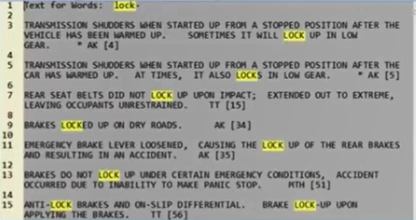
2. The Context in Text the Most Frequent Terms and Phrases are Used
Text explorer showing all sentences the selected term or phrases from the frequency table. User may explore the context the terms or phrases were used to better understand the issues buried in the expressions.
3. Terms or Documents Tend to Appear Together
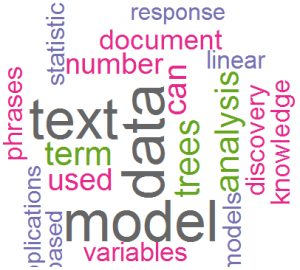
The “wordcloud” is a popular visual summary of the major theme of a body of text. Below is a word cloud constructed based on text in this blog homepage:
Wordcloud constructed based on words appeared in this web page. Certain stopping words were first removed, then TDM was constructed.
Terms or phrases in one document may also be clustered to fewer natural groups, as shown below:
Terms within a document may be clustered based on their proximity in meaning.
Terms or phrases within one cluster may be explored in the Word Cloud, to see how significant these are within the entire document.
Visual displaying a cluster of words within the entire document word cloud, which may offer a clue to the content of an important message that may not be discovered by classic supervised statistical methods.
Similarly, this may be done to cluster similar documents based on the terms or phrases that are dominant within each document.
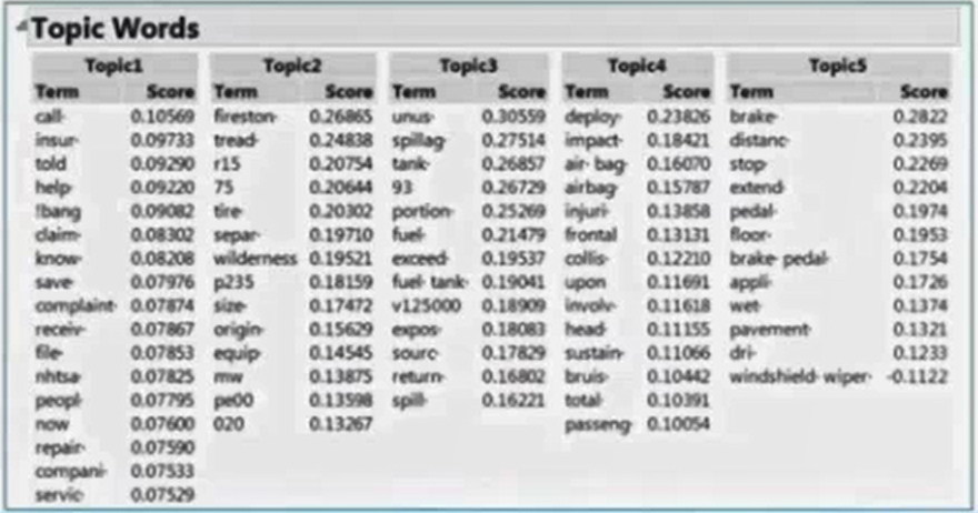
4. The Recurring Theme (Topics) in a Document
The terms grouped with in the topic provide a sense of the issue. Ranking of the terms tells user which topics are more important.
“Terms tend to go together” or Topics, is another way to uncover hidden information in text.
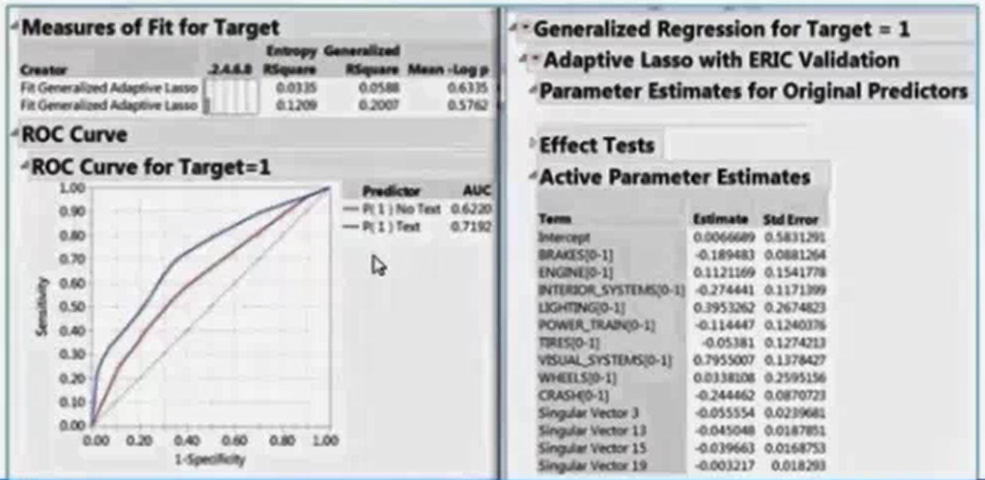
5. Singular Vector of Terms and the Predictive Power added to Prediction Models
Texting mining is mostly dimension reduction techniques of text data by associating words or phrases that appear in corpus. The build both descriptive and predictive models based on the reduced dimensions for understanding of the under cause or predicting future outcome.
Singular value decomposition (SVD) plot
Regression models may be conducted adding the singular vectors constructed based on the term and phrases in the documents. The top curve is the ROC curve shows the lift from the including of additional singular vectors, shown near the bottom right, upon using only the regular predictors, the second ROC from the top.
Terms and phrases singular vectors were added to the predictive model, shown in the lower right of the graph. As a result, the final ROC curve therefore the predictive power of the model is improved, the top curve vs. the second from the top.
Reviewing Concepts
Useful R packages for text analytics: R Packages ‘RcmdrPlugin.temis’ is a visual driven fast-result Text Analytics tool. As of June 2018 it is of Version 0.7.10. This ‘R Commander’ plug-in providing an integrated solution to perform a series of text mining tasks such as importing and cleaning a corpus, and analyses like terms and documents counts, vocabulary tables, terms co-occurrences and documents similarity measures, time series analysis, correspondence analysis and hierarchical clustering. Corpora can be imported from spreadsheet-like files, directories of raw text files, ‘Twitter’ queries, as well as from ‘Dow Jones Factiva’, ‘LexisNexis’, ‘Europresse’ and ‘Alceste’ files. The package provides different functions to summarize and visualize the corpus statistics. Correspondence analysis and hierarchical clustering can be performed on the corpus. Functions frequentTerms to list the most frequent terms of a corpus, specificTerms to list terms most associated with each document, subsetCorpusByTermsDlg to create a subset of the corpus. Term frequency, term co-occurrence, term dictionary, temporal evolution of occurrences or term time series, term metadata variables, and corpus temporal evolution are among the other very useful functions available in this package for text mining. R has a very rich set of analytic tools for text mining, though much in-depth knowledge may needed if one would like to become expert, these packages are summarized at here. (2017-11) A basic quick summary may be found here (2017-12)
Text analytics helps to discover original contents based on terms grouped in one cluster, and the story buried within. The capability of showing the text by clicking on the cluster is nice. Below text window displays all sentences of the words grouped within one cluster listed on lower left corner.
Ability to view the original document based on the grouped term cluster is an effective way to issue-discovery in text documents.
Text analytics is not just exploratory, with no significance measure or validation of results. It can also be used to linear models to understand the driving factor for certain outcomes. The “topics” summarized by the text analytics may be used as covariate variables, in the way principal components were used in certain regression analysis. So it is a dimension reduction technique. See the application example at the end.
Research Terms
Corpus: written texts, especially the entire works of a particular author or a body of writing on a particular subject, “the Darwinian corpus”. For software tools it is a collection of text documents, stored in a single data table column.
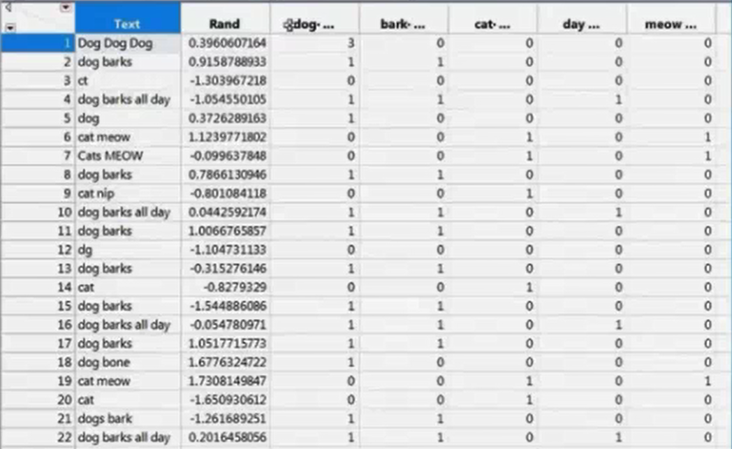
DTM (Document Term Matrix): A sparse matrix where columns correspond to terms, and rows correspond to documents. When a given document contains a given term, the corresponding cell is nonzero. There are several ways to assign values to non-zeros cells.
The Document Term Matrix format: each row is a document, each column is a term or phrase. The cells count the number of occurrence of the term within that document.
Tokenizing: The process of breaking a document into terms and phrases. Some software tool has functionalities for tokenizing that is also customization.
Stop Word: A term to be excluded from analysis. Software needs to have a built-in stop list which can be customized as desired.
Stemming: Treating terms with the same root as the same term. Example: “run”, “run” and “running” become “run”. Software needs to stem terms automatically, while also supporting customized exceptions.
TF IDF, the text analysis weighing term. Others are: Binary, Ternary, Frequency, Log Frequency
The way the terms are clustered
Latent Semantics Analysis, is the singular value decomposition (SVD) of the document and term matrix. SVDs account for most of the variability in the text, 80% of the SVDs are sufficient to almost all information
A “topic” is constructed. Topic formula can be saved for modeling. Clusters and latent classes can be constructed as categorical predictor, and singular vectors for continuous predictors.
Application Example
Analyzing car repair shop customer survey, to understand the car mechanical issues that made repair shop customers to change to a different manufacturer (churn rate) for their next car. Comment section of the customer survey is free expression section, car mechanic problem diagnostics are also free texts descriptions written by mechanics. Customer were as it they will change manufacturer, which is a Yes/No response. Final generalized model, used SVDs derived from text analytics of the customer and mechanics text descriptions as control variables. Each of SVD may be focused on certain aspects about how well the car was performing on.
The mean response level (% responded change next car manufacturer) versus the “topic” discovered by text analysis. This leads to a basic understanding of what drives the customers’ decision to change car manufacturer.
Decision trees may be called “classification tree” when the response is categorical, and “regression tree” when the response is continuous. The partitions are made to maximize the the distance between the proportions of the split groups with a response characteristic for classification tree, and to max. the difference of the means of the split groups for regression trees. Decision trees are user friendly and computer intensive methods therefore are well received with growing software popularity. The methods help users
Determine which factors impact the variability of a response,
Split the data to maximize dissimilarity or the two split groups,
Describe the potential cause-and-consequence relationships between variables
Decision trees split samples to maximize dissimilarity sequentially until no additional knowledge is gained.
Tree-based models avoids specifying model structure, such as the interaction terms, quadratic terms, variable transformations, or link functions etc. needed in linear modelling (though may be removed upon fitting the linear model model). It can also screen a large number, say hundreds of variables (linear models can use main effects to do the same, but may be error prone with too any variables) fairy quickly. It is user-friendly that computer does all the intensive computation, with minimal involvement of user knowledge in statistical theory (as in linear modelling).
Bootstrap forest (aka. Random forest) and boosted trees (aka. Gradient-boosted trees) are two major types of tree-based methods. Bootstrap forest estimates are averages of all tree estimates based on individual bootstrap samples (the “trees”). This averaging process is also know as “bagging”. Also the number of bootstrap samples, the sampling rate, the model which including the max. number of splits and the min. obs/node etc. are pre-specified.
On the other hand, boosted trees are layers of small trees built one-on-top-of-the-other, with smaller trees structured to fit the residuals from the top level tree. The overall fit improves as the residuals are minimized by adding smaller trees to fit the last model residuals. Both bootstrap forest and boosted tree methods may not be visualized directly, as these a complex tree structures. The most effective visual evaluation is through the model profiler available in software tools.
More data splitting results in better fit as measured by R-square. The graph below shows the increases in R-square in each splitting step, calculated separately on the training data (the top curve), the test data (orange) and the validations data (red):
improvement in R-square as the number of splits increases, but using the training data, the test data (orange) and the validations data (red)
At certain splitting step, the validation stops to improve, in this case, about the second or third step. The proportion of data select to use as validation data may affect the number of splits to be optimal, i.e., select 40% may ended with 3 splits to be the choice, vs. selecting 30% as validation that ended with 2 splits to be optimal (in other words, still an “art” not “science”)
Reviewing Concepts
The training and validation sets are used during training model. Once we finished training, then we may run multiple models against our test set and compare the accuracy between these models.
In some software tool, types of miss-classification may be controlled, by weighing the importance of Type I and Type II errors, specified as ratios in negative integers, larger the negativity, the more damage.
Research Term
“LogWorth”: the negative log of the p-value, the larger (or smaller the p-value, the more significance), the more it explains the variation in Y, is used to select among candidate variables the one split variable, and the value at which it splits the population. It is calculated as the negative log of the p-value
Application Example
May be used to select the most significant factor that separate workforce either by gender or race, i.e. job group, job function, geographic location, annual salary, bonus or job performance ratings.
Screen to a few among a large number of factors to use in design of experiment, to avoid the large number of expensive full or fractional experiment runs.
Though there are large number of variables may be used, only a few that will explain most of the variation in Y
(Modeling using JMP Partition, Bootstrap Forests and Boosted Trees)
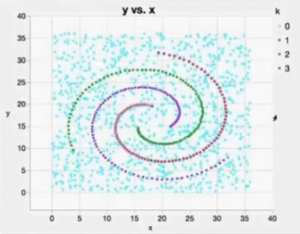
Neural Networks has the advantage of fitting responses of any shape or configuration, that usual analytic form can not or very hard to describe. See this 2-D spiral pattern, usual modeling technique will have a hard time to detect and fit the spirals, i.e. there no linear form that can be used to identify these spirals:
By fitting a Neural Network model we able to associate points on the plot to each of the three spirals.
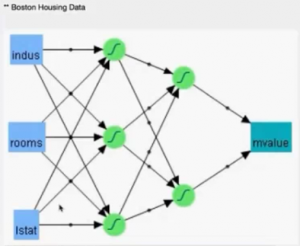
Neural Networks models also possess some sort of intuition or connection to everyday people’s understanding of cause and consequences. Factors and inner mechanism may be interrelated and opaque, but the inputs and results are mostly known and limited in numbers, see this example about understanding and therefore to predict future Boston area housing values:
The building of Neural Networks model is mostly composed by theses steps:
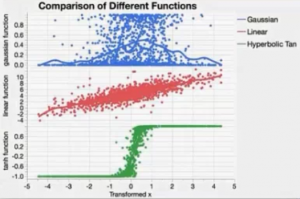
Activation functions and hidden layer structure: number of layers and number of nodes under each activation functions: TanH, Linear, and Gaussian, where
TanH: The hyperbolic tangent function is a sigmoid function (S-shaped, as logistic curves). TanH transforms values to be tween -1 and 1, and is the centered and scaled version of the logistic function
Linear: Most often used in conjunction with one of the non-linear activation functions. For example, place the linear activation function in the second layer, and the non-linear activation functions in the first layer. This would be useful if you want to first reduce the dimentionality of the X variables, and then have nonlinear model for the Y variables. For a continuous Y variable, if only Linear activation functions are used, the model for the y variable reduces to a linear combination of the X variables. For a nominal or ordinal Y variable, the model reduces to a logistic regression.
Gaussian: This function is used for responses display radial function behavior, or when the response surface is known as Gaussian (normal) in shape.Below is a comparison the fitting patterns for different data distributions from different activation functions:
Boosting: four important points to keep in mind.
Boosting is building a large additive neural network model by fitting a sequence of smaller models
and each of the smaller models fit on the scaled residuals of the previous model. The models are combined to form the larger final model
Boosting is often faster than fitting a single large model. However, the base model should be a 1 to 2 node single-layer model, or else the benefit of faster fitting can be lost if a large number of model is specified
The learning rate must be 0<1<=1. Learning rates close to 1 result in faster convergence on a final model, but also have a higher tendency to over-fit data. To specify a bigger learning rate will result in taking bigger learning steps in each iteration of boosting, smaller learning rate vice versa. The trade off is smaller learning rate will take longer time and may result in over-fitting, versus larger steps with faster completion but with likelihood of missing certain useful information. The usual learning rate to use is 0.01 (or 10%). Therefore the fitted model should be validated the same time it is boosted, i.e., stop boosting if the R-square from the validation model stopped from improving.
Fitting options: whether to transform the covariates, the penalty methods to choose, and the number of “tours”. Covariates may be transformed to normal; penalty may be taken to reflect the emphasis put on the covariates, choices are square, absolute deviation with weight decaying and no penalty; “tours” are the random start model fittings that ended with different model estimates, that are averaged to constructed the “ensemble model estimate
Search progression
Reviewing Concepts
Both input and output (response) variables could be either continuous or categorical.
Validation can prevent over-fitting, as over-fitted model tend not do well when using new data.
NN estimation starts with a random guess of the estimate, then the whole algorithm with improve until the best estimate at the end of the iterations. However the end estimate may be different depending on where the initial random guessing is. So the “ensemble method” takes a number of random starts, and the final estimate takes the average of the estimates.
The “confusion matrix” by number or rate may be convincing checking points; also the R-square on both the training and validation data ideally should be high and close to each other
The Confusion Matrices either by raw number cases or rates on both the training data set and the validation set are good quick evaluation of the value of the modeling effort.
Actual vs. Predicted plots both on the training and validation sets for continuous responses are a good visual aid (straight line) to exam model fitting
Closer the actual vs. predicted dots to the straight line the better the model fits
A “visual profiler” are useful to visualize the impact of each covariate on the response (probability of each category for category responses), under the fitted model, and how the changing of inputs one-at-a-time may impact the response, as well location of the inputs on at each level of the response
Example Multivariate Profiler of Fitted Model – How the Input and Responses and between the Response are Related
Nodes on the hidden layers are constructed in the way very similarly to principal components (PCs), i.e. reducing the high dimension of input nodes to one by expressing one linear combination of the inputs. NN builds the PCs along the way, but may not be linear
Statistical tools fitting the NN models should better be able to provide the final fitted formula so the model can be transported across platforms, say to Excel, SAS, Python, Java etc.
Working with “Regular Expression” (regex) is mostly “Pattern Matching”
Regex used in R may be found using “?regex” in R
dplyr
The “grammar of data manipulation”, a very useful extended basic functionality from basic R, worth very careful and skillful use of it, here is the link to the package doc.
tibble
Filter, Select, Create (mutate), Arrange (order by) columns, very much similar to Excel GUI process, consistent and easy to follow
dplyr, ggplot2, reshape2 as data scientist basic tools. “reshape2” mostly a data set transformation into usual analytical format, where SAS had been addressing for decades, see here for a basic intro.
Practical Challenges in Workforce Analysis
Search multiple Excel files, export rows containing particular regex (words group pattern) in any variable; also create a column that has the name of the Excel file so checks can be made if correction or further study are needed.
Select a column of a tibble based on regex pattern
Construct a meta data base with the basic identifier and all essential analysis variables. Or any variables that may be of interest for certain modeling requirement. This may be done by getting the file names (fileNames <- Sys.glob(“*.csv”)), then process the file by searching column names using regex
Challenges in creating these regex:
race status with variations of spelling, such as “White” vs “W”
keywords used in job title, or any classification similar to job title, such as job group, job function, but not department, i.e., “Research associate”
variable name that may indicating base salary, such as “Salary”, “Annual Salary”
Regex for
E-mail Addresses
Postal Codes
Telephone Numbers
Dates and Times
Social Security Numbers: this may be helpful, a little complicated
The meaning of “Advance” to commercial activities is equivalent to “Adding Value”, specially it is achieved through the following means:
Higher profits from offering product or services. Higher profit is achieved through selling product or services at higher prices, this means finding the product or services can be sold at higher prices in general, or locating the customer segments who are willing to pay for it, or both.
Lower cost in producing the product or services. Optimization of production or creation process may decrease costs in producing product or services. Optimization means better utilization of currently available resources, or finding alternative resources that cost less.
Discovery of new product or services that usually afford higher profit margin in early market offering stage where competition is rare, therefore beat the traditional competition,
Overcome road blocks in developing and maintaining products or services to meet contractual or bidding requirements,
Improvements of government service expected by the public.
Major statistical applications mentioned below can add commercial or governmental organizations to achieve these goals, in a way that are faster, and may not even be possible using traditional administrative or make-believe approaches, that non-specialists tend to regard as effective. Persons promoting these approaches to future clients should fully understand the clients problem, and the advantages of the mentioned below methodology over traditional methods.
The story may be long, but here is a broad overview. More detailed scenarios, applications or novel solutions may be expanded in future posts.
—————————————————
Data Mining, Machine Learning and AI
Organizations that will benefit:
How it adds value:
Scenarios:
Statistical Modeling
Organizations that will benefit:
How it adds value:
Scenarios:
Survey Research
Organizations that will benefit:
How it adds value:
Scenarios:
Discovery Methods, Innovation and Manufacturing Improvements